AMC Process Automation | Drill Planning & Budget Optimization

Drilling

Often the first budget item to be cut in times of austerity is the exploration drilling. We will not go into the wisdom or consequences of this decision, but rather look at a means to optimize the money available for on-going drilling. Most geologists who have had to do drillhole layouts will have come up with any number of tools or process automations through scripts or macros that help them design a reasonable drill plan in an acceptable time frame. One such approach is described in this article.

Drilling costs are generally broken down into mobilization, set-up, the unit drilling costs (per metre), logging, sampling, sample transport, and assaying and storage. Logging, sampling, and the other downstream activities tend to be set at fixed prices unless you are using contractors and ad hoc assay contracts. The biggest costs are therefore the drill collar set-up (pad or drilling station construction) and the drilling itself.

As such, if you have a constrained drilling budget then a balance between the number of drill pads and set-ups as well as the drill-metres required to achieve the campaign objectives needs to be found. Drilling the deposit to achieve an objective specification such as infill drilling is typically constructed around:

Targeted drilling to increase geological understanding;

Confirming continuity and minimizing geological risk through additional data and variations of this theme; or

Increasing and upgrading resources.

Designing a drill plan without a clear goal in mind or some sort of practical constraint on what can be completed and what is an acceptable outcome can result in a plan that, if executed, that will just burn money and not achieve the intended purpose.

A manual drill campaign planning approach (even with personal customizations and tools) can be a painful and laborious process. Even with a clear understanding of the drilling objectives it can be a significant challenge to generate a reasonable drill plan in the timeframe we are often given. Once the object of the drilling has been decided on, such as upgrading an Indicated resource to Measured, and the parameters that will limit the drilling (maximum hole length, minimum angles of intersection and drillhole spacing) the process of planning the drilling begins.

Drill planning

How do you do that? The general approach is to ignore the limiting factor of the drill pad or drill bay construction (often you have limited options from the get-go) and to iteratively layout holes in section and 3D while considering the existing drilling and spacing requirements. This basic approach seems to revolve around working in plan, cross-section or longitudinal (long) section and positioning the pierce points, then iteratively switch back and forth until we have the drilling layout. An example of this is given in Figure 1 where two phases of extensional drilling have been planned in long section.

The challenges inherent with this process is that it can be time consuming and is subject to individual bias. Combined with irregular or complicated drill spacing (Figure 2) this can be a very difficult exercise. Further challenges come from ensuring that the drill plan meets the requirements for maximum length of hole, rig capacities, intersection angles, and local and average pierce point spacing.

A manual, iterative process is not able to optimize the entire drill plan. It is limited to a hole-by-hole decision-making process that, due to the time required to complete, cannot be iteratively refined. The manual process, especially for short-term drilling that requires rapid turnaround on the planning, is subject to limited refinement beyond a default layout. This is not to say that the resulting plan is not achievable or effective. It might just not be the optimal use of the available budget or compromise the objective of the program.

How to

Consider the situation where the budget is severely constrained, drill set-up positions are limited and there is little time to complete the plan (all of us have been there at some time).

My initial approach to this was to develop a tool that laid out a theoretical intersection grid within the plane of the deposit and then randomly selected traces between the provided drilling positions and the intersections. While this approach was quick it did not always provide the best solution for a drill plan. The best plan being defined as a solution that gave the most spatial coverage for the least number of drill-metres and therefore the least expensive with the best return.

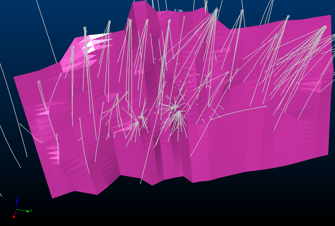
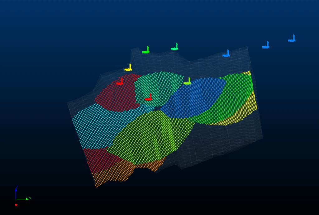
An interim output of this initial random drilling selection is shown in Figure 3. In this example, there are nine surface drilling positions and a steeply dipping narrow tabular deposit. Based on the non-ideal minimum intersection angles (45°) between the planned hole and the deposit local orientation as well as the selecting only the shortest holes, the roughly eye-shaped drilling footprints were calculated. It was from these restricted regularly spaced intersection points that the initial drill plan was selected.

This random selection approach results in hundreds of possible drilling configurations that may or may not be the best possible solution. The question then was how do I, with a limited drilling budget and no time, select the best possible configuration from all these options?

In many respects, this problem resembles the “travelling salesman problem” (TSP) which is defined as:

“The travelling salesman problem (TSP) asks the following question: “Given a list of cities and the distances between each pair of cities, what is the shortest possible route that visits each city exactly once and returns to the origin city?” It is an NP-hard problem in combinatorial optimization, important in operations research and theoretical computer science.” Wikipedia (2016).

Restating TSP for drill planning as follows:

What drilling configuration will give me the shortest set of holes that can be drilled by the equipment available, have the highest possible intersection angle and, on average, give the best infill coverage for the budget available all the while staying a minimum distance from existing or newly planned drillholes?

Due to the complexity of the problem it requires either tedious man-hours or some sort of algorithm. There are any number of optimization algorithms out there (hill climbing, genetic algorithms etc.). For this solution, simulated annealing was chosen as the optimization approach as it was the simplest to implement in the timeframe available.

How it works

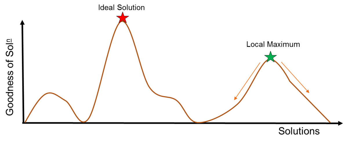
In general, an optimization algorithm randomly selects an initial solution. It then randomly selects a second solution and if it is better than the first, it switches to the second, and repeats until the algorithm finds a maximum solution. But these can be trapped at local maxima. Solutions that are locally good but not the best. This is schematically illustrated in Figure 4.

Simulated annealing avoids this “trap” by adding a random component to the decision to switch.

Relying heavily on the work of Geltman (2014) a simulated annealing algorithm was developed. The basic process can be summarized (from Geltman, 2014) as:

First, generate a random solution.
Calculate its cost using some cost function you have defined.
Generate a random neighbouring solution.
Calculate the new solution’s cost.
Compare them: a) If cnew < cold: move to the new solution b) If cnew > cold: maybe move to the new solution
Repeat steps 3-5 above until an acceptable solution is found or you reach some maximum number of iterations.
“When calculating if a solution is better it calculates an acceptability probability (Ap)”
𝐴𝑝=𝑒^((𝑜𝑙𝑑−𝑛𝑒𝑤)/𝑇)

Key to the calculation is the use of (T) or the annealing temperature and is a decrementing value starting at 1 which allows the process to move from a random solution to an optimal or minimized solution.

If the acceptability probability is equal to zero then the new solution is infinitely worse, and is rejected. If the Ap value is equal to one then the new solution is infinitely better and is automatically selected. For values between zero and one, the Ap value is compared to a random value (Rv). If it is greater than the Rv, the new solution is kept, otherwise it is rejected.

In this manner, at decreasing T values, a solution must be dramatically better than the current solution to be kept, except that the random function means that a potentially worse local solution can be selected. This is the key to not getting stuck at local maxima.

The working solution

My solution uses an implementation of this simulated annealing algorithm. Key to its function is the ability to calculate the intersection angle between the drillhole and the orebody to ensure the steepest and therefore optimum intersection angle possible. It also allows control over the drilling dip, maximum hole length, and total drilling budget as defined by a total number of metres to be drilled.

Further inputs are the initial geological model, any existing holes, as well as any existing mining voids. By using the existing drilling and mining data, the tool ensures that the planned drilling does not come within a specified distance of existing holes (unnecessary over-drilling) or of existing voids (safety).

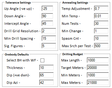
An extract from the control interface is shown in Figure 5 where the control settings for the drillholes, the simulated annealing algorithm, and the drilling budget are detailed.

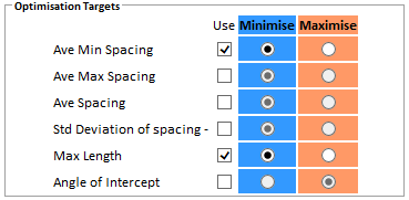
Key to the implementation is the definition of the cost function (e.g. average hole length) against which each of the randomly constructed drilling plans are measured. It must be noted that the cost function is not a direct financial cost, rather a mathematical expression of value as a function of one or more parameters. Figure 6 shows the six possible optimization targets (“cost functions”) that can be selected. Minimizing the standard deviation of the planned hole spacing will result in holes clustering around each other at the minimum specified spacing. Maximizing the standard deviation will force the holes to disperse as widely as possible within the constraints of the minimum allowable intersection angle, drill rig operating parameters and maximum hole length.

Drilling checklist for mining optimization

The tool also allows for the simultaneous design of both an underground and surface drilling programme (provided they share a budget for drilling metres).

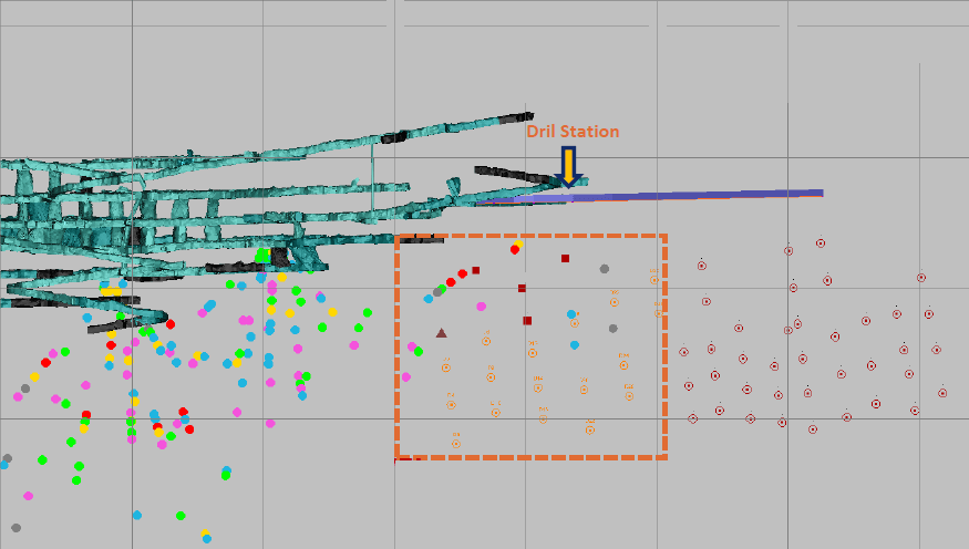
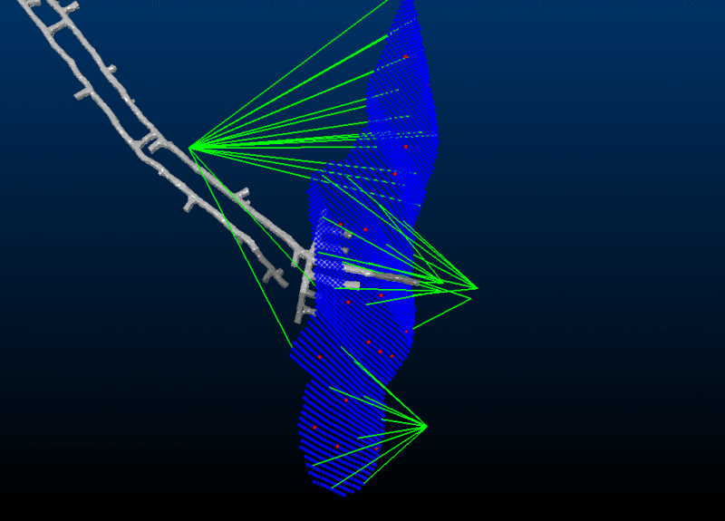
We have used this tool to efficiently layout underground drill programmes with limited drilling positions in both the hangingwall and footwall of deposits. The tool effectively constrains the “drillable” area and ensures that the drilling spacing is correct and that no unrealistic up holes are planned as had happened previously during manual layout in the same areas. An example of an underground drilling plan is show in Figure 7 where 23 holes have been laid out on a 5 m × 5 m intersection grid with no hole steeper than 20° up and no closer than 30 m from any existing or planned hole.

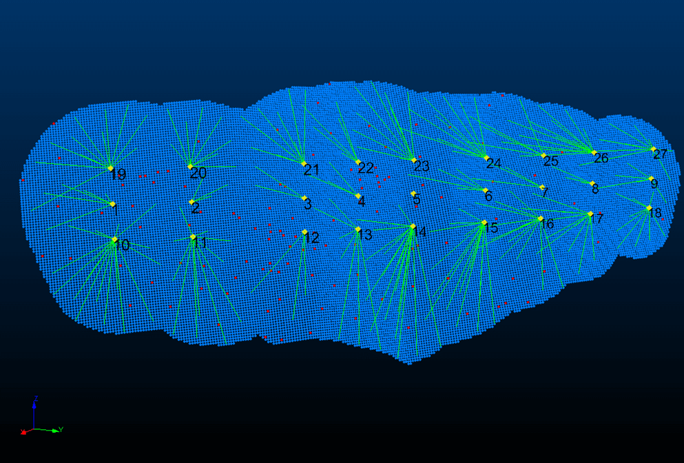
The tool has also shown itself to be very effective at laying out grade control drilling rapidly and reasonably as shown in the synthetic example in Figure 8. The total time to layout these 200 plus holes was less than ten minutes.

Computerized drill plan for budget optimization

Conclusion

The implementation of this algorithm allows the user to test many possible but potentially sub-optimal drillhole layouts within a few minutes to produce a robust, achievable, drilling plan within the specified budget, for the desired objective, and constrained by the configuration or layout specification.

There are some refinements still required. The algorithm needs to be further tested and the ranking of the various cost functions (spacing, average length etc.) needs to be adjusted as it is currently hardcoded in the order shown in Figure 6. Further tweaking is required to minimize the number of drilling stations used and to allow the individual drilling rig controlling parameters to be set on the collar rather than having simple global defaults.

While the tool can test an existing drilling plan in general terms by working with the specified budget and planned collar positions, the next stage is to be able to load the drill plan as the first “random” scenario to the optimization process and use the simulated annealing algorithm to test the robustness of the manual design.

This tool is aimed at aiding a geologist, generating the optimal design that is going to maximize the available drilling budget according to the resource classification or grade control requirements of that specific site.

References

Geltman, K.E. (2016), The Simulated Annealing Algorithm, web, http://katrinaeg.com/simulated-annealing.html, Last Accessed: June 2017.
Wikipedia, Travelling salesman problem, web, https://en.wikipedia.org/wiki/Travelling_salesman_problem, Last Accessed: June 2017
Text by Justin Glanvill
Subscribe for the latest news & events